Rebuilding Housing in Harvey’s Aftermath: Two Lessons from Hurricanes Katrina and Rita

by Jonathan Spader
Senior Research Associate

As floodwaters finally subside in Houston, and as Florida residents prepare for Irma, residents, civic leaders, and policymakers can glean two important lessons from the intensive efforts to rebuild homes and communities after Hurricanes Katrina and Rita, two devastating storms that hit the U.S. in back-to-back succession in 2005. 

First, rebuilding residential properties is a lengthy process likely to take several years. Second, the rebuilding process will be especially lengthy for rental properties (as compared to owner-occupied homes), which could greatly affect the 950,000 renters (who account for 41 percent of households) in the greater Houston metropolitan area, as well as additional renters affected by Hurricane Harvey in elsewhere in Texas and in other states. The slower pace of rental rebuilding is due to several factors including both renters’ dependence on property owners to rebuild rental housing units and historical differences in the availability and terms of federal aid for rental property owners as compared to homeowners.

To be sure, the need for emergency assistance and shelter for displaced residents will continue for weeks to come. Nevertheless, Congress is already starting to discuss an aid package. Moreover, the extensive damage (and the need to reauthorize the National Flood Insurance Program before September 30) may spur new efforts to develop policies and programs to support housing recovery in the wake of future natural disasters. As policymakers, civic leaders, and local residents begin to focus on the rebuilding process, they might want to keep the following in mind.

Extensive flooding from Hurricane Harvey in Southeast Texas. Air National Guard photo by Staff Sgt. Daniel J. Martinez

1. Rebuilding residential properties takes time.

An initial lesson from Hurricanes Katrina and Rita is that the rebuilding process takes time, with many properties continuing to show observable damage several years after the storms had passed. In early 2010—almost five years after both hurricanes made landfall—a HUD-commissioned study that I worked on surveyed the exterior conditions of properties damaged by those storms. The survey produced representative estimates of the rebuilding outcomes of properties that experienced “major” or “severe” damage—defined by FEMA as $5,200 or more in storm-related damage—that were located on significantly-affected blocks—defined as a city block on which three or more properties experienced “major” or “severe” damage.

The survey found that 17 percent of hurricane-damaged properties in Louisiana and Mississippi still showed substantial repair needs as of early 2010, almost five years after the storms had hit. Almost half these properties did not meet the U.S. Census Bureau’s definition of a “habitable structure,” a housing unit that is closed to the elements with an intact roof, windows, and doors and does not show any positive evidence (e.g. a sign on the house) stating that the unit was condemned or was going to be demolished. Only 70 percent of hurricane-damaged properties in Louisiana and Mississippi were rebuilt by early 2010, and 13 percent contained cleared lots in which the damaged property had been removed from the parcel (Figure 1).

In the case of Hurricanes Katrina and Rita, the properties that still were damaged included some whose owners had received rebuilding grants through federal programs designed to aid housing recovery. The largest source of assistance following the 2005 hurricanes was the $18.9 billion special Community Development Block Grant (CDBG) appropriations passed by Congress between 2005 and 2008. Some portion of the properties with remaining damage likely also reflect abandonment by owners who moved elsewhere in the wake of the hurricanes. For such properties, funding for demolition, rehabilitation, and land banking may be necessary to transition the properties to a new use, and potentially to support efforts to encourage residents to rebuild in areas with lower flood risks.

Notes: Sample is representative of properties in Louisiana and Mississippi that experienced major or severe hurricane damage and that were located on significantly-affected blocks. Rebuilt structures are residential structures that do not show substantial repair needs as defined in Turnham (2010). Cleared lots contain an empty lot or a foundation with no standing structure. Damaged structures are residential structures that show substantial repair needs—and include all uninhabitable structures. Uninhabitable structures are residential structures that do not meet the Census definition of habitability. 

Source: Spader (2015).

2. Rental properties were rebuilt more slowly than homeowner properties.

A second lesson from the rebuilding process following Hurricanes Katrina and Rita is that rental properties were rebuilt more slowly than owner-occupied homes. This likely was due to several factors. While homeowners directly control the rebuilding progress of their home, renters are dependent on landlords’ rebuilding decisions. Smaller “mom-and-pop” landlords may also be slower to rebuild investment properties if their own home is also damaged. And policymakers have been wary of providing rebuilding assistance to rental property owners who did not purchase sufficient insurance.

Following Hurricanes Katrina and Rita, both Louisiana and Mississippi used the CDBG special appropriations for disaster recovery to create rebuilding assistance programs for homeowners and small rental property owners. (Texas, which faced less damage from Hurricanes Katrina and Rita, created only a homeowner program.) In both Louisiana and Mississippi, the homeowner programs covered much of the difference between the estimated cost to rebuild and the amount available to the homeowner from insurance and other rebuilding-assistance programs. Conversely, the grant programs for 1-4 unit small rental properties included a more complex set of eligibility requirements that included commitments for the rebuilt units to be rented to qualifying low- and moderate-income tenants. The result was that few rental property owners applied for and received rebuilding assistance, compared to widespread take-up of the homeowner assistance programs. While concerns about the incentive effects associated with bailing out under-insured investors are reasonable, a secondary effect was to reduce the number of rebuilt properties available to renters.

Figure 2 displays the share of hurricane-damaged properties on significantly-affected blocks that received a rebuilding grant through the CDBG-funded homeowner and small rental programs, along with the share of homeowner and small rental properties that were rebuilt by early 2010. The results show that 58 percent of hurricane-damaged homeowner properties in Louisiana and Mississippi received a rebuilding grant, compared to 10 percent of small rental properties. While this rental figure is limited to 1-4 unit small rental properties, a GAO report similarly found that federal assistance through CDBG, the Individual and Households Program, and the Home Disaster Loan Program together reached only 18 percent of all damaged rental units (including units in larger multi-family buildings), compared to 62 percent of damaged homeowner units. The rebuilding outcomes documented in the HUD-commissioned survey also showed sizable gaps, with 74 percent of homeowner properties rebuilt by early 2010 compared to 60 percent of rental properties.

 Source: Spader and Turnham (2014); Spader (2015)

A final question for policymakers is whether to use this opportunity to create a permanent program to support housing recovery following natural disasters. While Congress has relied on the CDBG program for this purpose since the early 1990s, its role is currently defined by the special appropriations legislation drafted following each individual disaster. Making disaster recovery a permanent function of the CDBG program (or creating some other permanent program for housing recovery) would allow HUD to develop permanent regulations and program guidance in anticipation of future disasters. While it is too late for this change to benefit victims of Hurricane Harvey, it might improve preparedness for the next disaster.

Defining the Generations Redux

by George Masnick
Senior Research Fellow

How should we define the baby boom, Generation X, and the millennial generation?

In a Joint Center blog published in 2012, I argued that using 20-year age spans for each generation would make it easier to compare them. Since many researchers still use generational definitions that span different and inconsistent age ranges, particularly for millennials, it is perhaps timely to reframe and restate my case.

In keeping with my recommendations, the Joint Center has long identified the cohort born between 1945 and 1964 as baby boomers.Those born between 1965 and 1984 are Generation X, and the cohort born between 1985 and 2004 are millennials (Figure 1). 

However, other analysts use several different earlier dates to usher in the millennial generation, apparently because they want to ensure that the oldest member of this cohort were considered adults at the dawn of the new millennium (i.e. they had turned 18 or 20 in the year 2000). This definition meant that by 2015, the oldest millennials were in their mid-30s, old enough to prompt compelling stories about how many 30-somethings were still living with parents, living in cities, forsaking marriage and childbearing, and delaying homeownership. In contrast, under my recommended cut-off dates, the oldest millennials turned age 20 in 2005 and didn’t start entering their 30s until 2015.

Besides making it easier to compare generations, there are several reasons why the millennial generation should start with those born in 1985 and turning 20 in 2005. As I noted in my 2012 blog, 1985 was the year that U.S. births once again exceeded 3.7 million, the approximate number that demarcated the beginning and the end of the baby boom, as well as the beginning and the end of the “baby bust” that defines Generation X.

Three other big changes occurred shortly after 2005 that significantly altered the way young adults live. First, social media participation skyrocketed. Facebook became available to everyone age 13 and older with a valid e-mail address in September 2006. Twitter became public in 2006. The first iPhone was released in June of 2007. As a result of these and other changes, the share of adults using social media rose from five percent in 2005 to 69 percent in 2016, according to a recent Pew Research publication.

Second, student loan debt outstanding more than tripled between 2005 and 2016, rising from $400 billion to over $1.3 trillion. This high level of debt is thought to affect everything from leaving the parental home, to getting married and starting a family, and purchasing a first home. 

Third, and perhaps most importantly, the economic changes that led to the Great Recession hit hardest among young adults who were in their 20s shortly after 2005. The unemployment rate of adults older than 25 without a high school degree rose from below six percent in late 2006 to 15 percent in mid-2009. (Those with a high school degree or more followed this trend within a year.) Unemployment rates of those with a high school degree or more have slowly improved, but still remain above pre-recession levels. Unemployment rates for those with less than a high school degree have returned to their pre-recession elevated levels, but people in this group generally are making less money and receiving fewer benefits than they did before the recession. Meanwhile, housing costs have returned to, or now exceed, their pre-recession levels.

Using equally broad 20-year age spans produces several important findings about the different generations. To start with, the millennial generation has been larger than the baby boom generation, now or at any other previous time since the boomers were age 10-29 in 1975 (Figure 2). Millennials now number almost 87 million compared to less than 79 million for baby boomers at the same age. This is in contrast to findings of a 2016 Pew Research study that compared generations using millennials with a smaller age range and found roughly equal numbers between these two generations in 2015 (75 million).

Source: Census Bureau Population Estimates 1975-2015

Using consistent age spans also shows the changing ways that immigration has affected the number of people in each generation. In 1995, when Generation X was age 10-29, it was smaller than the baby boom generation was in 1955, when it was the same age. However, because of immigration, by 2005, when Generation X was age 20-39, it already exceeded the number of baby boomers at the same age. 

Immigrants also make up a small but growing share of millennials. In 2015, 9.6 percent of millennials were foreign born compared to 21.4 percent of Generation X, and 15.3 percent of baby boomers (Figure 3). However, according to the latest Census Bureau population projections, the share of millennials who are foreign born is expected to rise to 20.9 percent in 2035 when they are age 30-49, which will boost the number of millennials to 97.3 million (Figure 4).  

Source: Census Bureau Population Projections for 2015

* Data do not allow 85-89 year olds from 85+ age group

Source: Census Bureau Population Projections for 2035

Finally, the constant-age-span approach allows us to identify significant generational differences in race and ethnicity. Overall, in 2015, 45.4 percent of millennials, 41 percent of Generation X, and 28.6 percent of baby boomers were minorities (i.e. non-Hispanic Blacks, non-Hispanic Asian/Others, or Hispanics of any race). Moreover, because of continued immigration, the share of millennials who are minorities is projected to rise to almost 50 percent in 2035 and the share of Generation X is projected to rise slightly to 42.4 percent. In contrast, the share of baby boomers who are minorities is projected to hold constant at 28.6 percent. 

These differences reflect changes for both foreign-born and native-born members of each generation. In 2015, fully 85 percent of both foreign-born millennials and foreign-born members of Generation X were minorities.  In contrast, only 78.5 percent of foreign-born baby boomers were minorities. Moreover, while 41.2 percent of native-born millennials were minorities, only 29 percent of native-born members of Generation X and 19.6 percent of native-born baby boomers were minorities (Figure 5).

* Data do not allow 85-89 year olds from 85+ age group

Source: Census Bureau Population Projections

Looking forward to 2035, the size of the baby boom cohort will drop to about 60 million people because a growing number of baby boomers will pass away. Many millennials and members of Generation X will want to live in the housing units formerly occupied by those baby boomers. Their ability to do so will not only be shaped by the fundamental economic and social changes discussed above but also by whether the large numbers of racial and ethnic minorities in these two generations will have full access to those housing markets, and with it, the ability to achieve the American dream. 

Homeownership Rates for Children of Immigrants—Age Matters

by George Masnick
Senior Research Fellow

Analyses of data used in a recent Census Bureau report show that homeownership rates for younger adult children of immigrants are substantially higher than rates for immigrants in the same age cohorts. In addition, while homeownership rates for native-born residents with native-born parents under age 45 are higher than those for the children of immigrants, members of the latter group quickly make up this deficit after the age of 45.

These findings emerge from additional analyses of data used in a first-ever report on the characteristics of three generations of US residents by nativity that was released late last month by the Census Bureau. The report is the first to use a unique question in the Current Population Survey‘s Annual Social and Economic Supplement (CPS/ASEC) asking the birthplace of both the respondent and the respondent’s parents. This allows one to identify people born abroad (1st generation), native-born children of at least one immigrant parent (2nd generation), and those whose parents were both born in the United States (3rd-and-higher generations).

The Census report discusses differences among the three groups in such areas as age, education, labor force participation, income, poverty, occupation, and homeownership. The last section is particularly interesting because other Census Bureau data the Joint Center has used to study homeownership, such as the Decennial Census, the American Community Survey, and the American Housing Survey, do not ask respondents where their parents were born. Moreover, as I have shown in an earlier post that also used CPS/ASEC data, immigrants are an important part of a recovering housing market. Foreign-born people have accounted for about one-third of all net household formations over the past two decades, and slightly under 30 percent of all gains in owner-occupied housing. Fully half of all household growth between 1994 and 2014 by under-30-year-olds came from 2nd generation children of immigrants, and another 35 percent from immigrants themselves.

The Census Bureau report notes that incomes and homeownership rise sharply between the 1st and 2nd generations but tend to level off for the 3rd-and-higher-generations. However, these findings may obscure significant differences between the 2nd and 3rd-plus generations because, as other parts of the Census Bureau report note, the generations have dramatically different age distributions. In particular, the majority of immigrants are middle-aged, and their children are 20 or younger. Adult children of immigrants have their largest percentages in the under-30 age group. Baby boomers dominate the 3rd-and-higher generations at age 50-70 in 2013 (Figure 1).

Source: U.S. Census Bureau, Characteristics of the U.S. Population by Generational Status: 2013, Current Population Survey Reports, Nov. 2016, Figure 9.

Because of these differences in age structure, it is impossible to compare the three generations broadly on any variable that varies with age, such as income or homeownership. For example, as the Census report shows, the median income among all individuals age 15 and over rises dramatically from $36,669 for the 1st generation to $46,764 for the 2nd generation. But, at $46,795, it is virtually unchanged for the 3rd-and-higher generations. However, when the data are broken down by age groups, they tell a somewhat different story. The Census report, which looks at median personal income for four broad age groups, shows significant income advantages for the 2nd generation over the 3rd-and-higher generations for 25-44, 45-64, and 65+ year olds. When median household income (a more relevant definition of income with respect to homeownership) is broken down into 5-year age groups, the 2nd generation can be seen to earn significantly more than their parent’s generation at every age, and importantly, more than the 3rd-and higher-generations as well (Figure 2).

Source: Joint Center for Housing Studies tabulation of 2015 CPS/ASEC data.

The need to control for age is especially important when examining generational differences in homeownership. In four of the five household family types discussed in the Census report, when age is not controlled, 2nd generation homeownership rates are lower than those for the 3rd-and-higher generations (and in the fifth, the difference between the groups is quite small) (Figure 3).

Source: U.S. Census Bureau, Characteristics of the U.S. Population by Generational Status: 2013, Current Population Survey Reports, Nov. 2016, Fig. 28.

If we control for age, would 2nd generation homeownership rates still be lower than those for the 3rd-and-higher generations? Also, since the Census report examined generational differences for a single year (2013), if there are differences by age, how well have they held up over time?

To answer these questions, we examined homeownership rates by age by 5-year age groups for the three generations for each year 1994-2015. These tabulations first can be summarized by examining the trends for two broad age groups (Figures 4 and 5). For households age 25-44, 2nd generation homeownership rates are well above those of their parents’ generation but below those of the later generations. This last pattern is partly explained by the greater concentration of younger 25-34 year olds in the broader 25-44 age group for the 2nd generation, and probably also due to the greater concentration of immigrants and their children in locations that have below average homeownership rates, such as the Los Angeles, San Francisco, New York City, Boston, and Chicago metropolitan areas. There might also be a greater ability of 3rd-and-higher generation parents to help their children financially in buying their first home, and a corresponding need for children of immigrants to save longer for a downpayment.

Source: Joint Center for Housing Studies tabulations of 1994 through 2015 CPS/ASEC data.

Source: Joint Center for Housing Studies tabulations of 1994 through 2015 CPS/ASEC data.

This analysis also shows that among younger adults the gap between the homeownership rates of the 2nd and 3rd-and-higher generations has widened since the Great Recession. The growing gap might be due to compositional shifts within the broad 20-year age cohort in such factors as age, ethnic composition, household composition and income. Alternatively, tightening credit markets might affect the generations differently. This could be particularly important for undocumented members of the 2nd generation. In any case, both the generational gap for younger adults and their recent trend certainly deserve further investigation.

For the broad adult age group over age 45, the story is quite different. Among older adults, the homeownership rates among the 2nd and 3rd-and-higher generations have been essentially equal for the past two decades except for a few years at the height of the Great Recession. The slower entry into homeownership we noted for younger 2nd generation households appears to have simply reflected the timing of the transition from renting to owning, rather than the effects of any structural differences between these two generations. After age 45, the 2nd generation has consistently closed the gap with the 3rd-and-higher over the past two decades. Another way to look at this homeownership data is to follow different birth cohorts of young adults as they age from the 25-44 age group into the 45-64 group. For each of the five-year 2nd generation cohorts under age 45 in 1995, the homeownership rates are lower than the respective cohorts in the 3rd-and-higher-generations. However, by 2015, when each of these cohorts is 20 years older, the homeownership gap between the generations has been completely eliminated (Figures 6 and 7).

Source: Joint Center for Housing Studies tabulations of 1995 CPS/ASEC data.

Source: Joint Center for Housing Studies tabulations of 1995 CPS/ASEC data.

The higher median income of 2nd generation adults above age 45 perhaps provides just the leverage they needed to make up the lost ground. And it is also likely that the older 2nd generation households are more concentrated in locations that have lower homeownership rates than the national average. If we could control for metropolitan location as well, middle-aged 2nd generation age-specific homeownership might well be higher than for the 3rd-and-higher generations. Unfortunately, the CPS/ASEC sample size does not allow such sub-national trends to be observed.

In sum, it is important to underscore that failing to recognize the important age differences between the three generations can lead to erroneous conclusions about levels and trends in income and homeownership. Because the 2nd generation age structure is so young, comparisons that lump adults of all ages together will result in unduly low incomes and homeownership for this group. As the Census report concludes, most 2nd generation U.S. residents surpass their parents’ generation in many measures, particularly education, income and homeownership. Once proper age controls are introduced, they equal or surpass the 3rd-and-higher generations in these dimensions as well.

Projection: US Will Add 25 Million Households by 2035

by Dan McCue
Senior Research Associate

The United States will add 13.6 million households between 2015 and 2025 and another 11.5 million households between 2025 and 2035, according to Updated Household Projections, 2015-2035: Methodology and Results, a new Joint Center working paper. This growth represents an increase from the past decade that is in line with historic rates of growth seen in the 1990s, but still well below the levels experienced in the 1970s (Figure 1). An addendum to the paper indicates that the projected growth in households could lead to continued growth in residential construction activity.

Sources: JCHS Tabulations of US Census Bureau, Housing Vacancy Surveys, Decennial Censuses, and 2016 JCHS Household Projections  

The new household projections incorporate newer population projections from the US Census Bureau that are substantially larger than the Bureau’s 2012 population projections used in our 2013 estimates of household growth, which projected that the U.S. would add 12.4 million households between 2015 and 2025 and 10.35 million households between 2025 and 2035. Our new household projections also make methodological changes related to headship rates—the ratio of households to people—designed to reflect the fact that shifts in headship rates have significantly impacted household growth over the past decade. (As the paper discusses in more detail, rather than continuing the Joint Center's recent practice of holding current headship rates constant, the new estimates use trended headship rates.)

While both changes are significant, the increases from our 2013 household projections are due entirely to the new Census Bureau population projections. In contrast, the methodological changes produce slightly lower projected growth than our previous methodology. However, the methodological changes do affect the distribution of household growth by age, race and ethnicity. In particular, they increase household growth among the oldest age groups and also among non-Hispanic whites between 2015 and 2025. In contrast, they reduce growth among 25-44 year olds as well as from black and Hispanic households.

Despite these shifts, millennials and minority households are still projected to be the main drivers of household growth in coming decades. Indeed, millennials under age of 30 in 2015 are projected to form 23 million net new households between 2015 and 2025, while 72 percent of household growth overall is expected to be non-white households. At the same time, aging of the baby boom generation will bring the number of senior households up to unprecedented heights (Figure 2). Together these forces will reshape housing demand over the next two decades.

Source: 2016 JCHS Household Projections

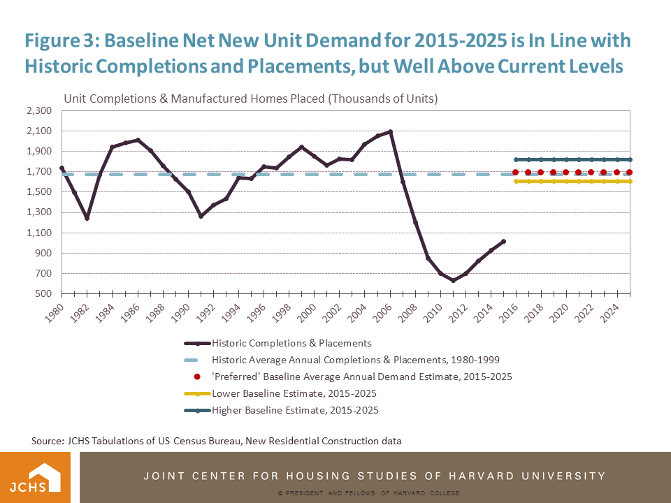
In addition to the estimates on household growth, the working paper includes an addendum with baseline estimates for the amount of new residential construction that might be needed to accommodate future household growth, as well as the demand for replacement units, second homes, and other changes. Combined, these factors suggest that the baseline demand for new housing units between 2015 and 2025 will range from 16.0 to 18.2 million units. While this estimate is well above most recent rates of new unit completions and mobile home placements, it is consistent with historic averages for past 10-year periods (Figure 3). Although the analysis does not factor in estimates of over- or under- supply, the estimates do suggest underlying demand will support higher construction levels and that the growth in residential construction seen over the past five years is likely to continue.

Source: JCHS Tabulations of US Census Bureau, New Residential Construction data

Read the full working paper: Updated Household Projections, 2015-2035: Methodology and Results,

Three Scenarios for the Future of Homeownership Rates

by Jonathan Spader
Senior Research Associate

Following the rise and fall in the homeownership rate over the past two decades, considerable uncertainty exists about the homeownership rate’s future trajectory. In a new working paper, I present three plausible scenarios and examine the implications of different homeownership rate outcomes for future growth in the number of homeowner and renter households. (A supplemental working paper provides additional analysis of the factors that have contributed to the homeownership rate’s decade-long decline.)

The tenure projections for growth in the number of homeowner and renter households through 2035 build directly on household growth projections also released by the Joint Center this week. We use these household growth estimates, along with data on homeownership rates from the Census Bureau’s Annual Social and Economic Supplement to the Current Population Survey (CPS/ASEC), to construct three scenarios that reflect a range of possible homeownership outcomes.

• Scenario 1 (“Base Scenario”) – Constant homeownership rates. The base scenario applies the 2015 homeownership rates by age, race/ethnicity, and family type to the projected household counts for each year. This scenario therefore describes the likely outcomes if homeownership rates stabilize near their current levels. By holding homeownership rates constant, this scenario also reveals the implications of changes in the distribution of U.S. households by age, race/ethnicity, and family type for the future homeownership rate.
• Scenario 2 (“Low Scenario”) – Continued decline through 2020 followed by constant homeownership rates. The starting point for the low scenario is the set of 2015 homeownership rates for each age, race/ethnicity, and family type category. The low scenario then projects the 2020 rates for each category by applying the 5-year cohort trends observed from 2010-2015. The 2020 homeownership rates for each age, race/ethnicity, and family type category are then held constant to project the homeownership rates for 2025, 2030, and 2035. This scenario describes the likely homeownership outcomes if the homeownership rate’s ongoing decline continues for several more years before stabilizing.
• Scenario 3 (“High Scenario”) – Homeownership rates return to pre-boom levels. The third scenario applies constant homeownership rates determined by the maximum of the 1995 and the 2015 rate for each age, race/ethnicity, and family type category. This scenario uses the 1995 homeownership rates to define the pre-boom levels that might reflect a longer-term equilibrium. It then adjusts the rates upward to the 2015 rates for older households and other groups for whom longer-term upward trends have kept the 2015 rates above their 1995 levels. The resulting homeownership rates therefore define a high scenario in which homeownership rates increase to levels slightly above than their 1995 levels, but well below their mid-2000s peaks. While such homeownership rate increases may be more plausible over longer-term periods than in the next few years, the high scenario applies these rates to all time periods, providing estimates of homeowner growth if the rates are realized within each time horizon.

The base scenario shows that changes in the distribution of households by age, race/ethnicity, and family type will not substantially alter the homeownership rate between 2015 and 2035. Rather, the homeownership rate would increase slightly from 63.5 percent in 2015 to 63.7 percent in 2025 before falling to 63.3 percent in 2035. (Figure 1) Because the base scenario holds the rates for each age, race/ethnicity, and family type category constant at their 2015 levels, the changes (or lack thereof) reflect the cumulative effect of trends in the profile of U.S. households, such as population aging, increased racial and ethnic diversity, and delayed marriage and childbirth. The upshot is that these trends largely offset one another, affecting the overall homeownership rate only minimally. Instead, increases in the number of homeowner and renter households are driven by household growth, producing 8.9 million additional homeowner households and 4.7 million additional renter households by 2025, and 15.7 million additional homeowner households and 9.4 million additional renter households by 2035. (Figures 2 and 3)

Source: JCHS tabulations of CPS ASEC data

Source: JCHS tabulations of CPS ASEC data

Source: JCHS tabulations of CPS ASEC data

While the base scenario’s projections halt the decade-long decline in the homeownership rate, the projected homeownership rates remain below their levels between 1985 and 2015. This partial recovery reflects the possibility that slowing foreclosures and a strengthening economy will ease the downward pressure on the homeownership rate in coming years, while also allowing for the foreclosure crisis and Great Recession to carry some lasting impacts. The relative importance of these offsetting pressures will only be known with time, so the base scenario’s projections should be interpreted as a reference point for homeownership outcomes if the overall rate stabilizes around its 2015 level.

The low scenario describes the consequences of continued declines through 2020 before the homeownership rate stabilizes. Under this scenario, the projected homeownership rate falls from 63.5 percent in 2015 to 60.7 percent in 2020 before leveling off at 60.8 percent in 2025 and 60.6 percent in 2035. The homeowner growth figures show that the continuation of the 2010-2015 cohort trend implies minimal growth in the number of homeowner households, adding just 755,471 additional homeowner households through 2020. In subsequent years, the eventual stabilization of the homeownership rate at 2020 levels allows household growth to add 4.9 million homeowner households through 2025 and 11.6 million homeowner households through 2035. This sluggish growth in homeowner households is accompanied by faster increases in the number of renter households, with 8.7 million additional renter households by 2025 and 13.5 million additional renter households by 2035.

The projected declines in the homeownership rate through 2020 reflects the replication of recent cohort trends from the starting point of cohorts’ already-low 2015 homeownership rates. The projected 2020 rates therefore assume a continuation of the foreclosure-related homeownership exits, tight credit conditions, weak incomes, and other factors that contributed to the homeownership rate’s recent declines. Additionally, they assume the absence of any catch-up growth due to pent up demand among households unable to buy a home in recent years or to homeownership reentries among households that experienced a foreclosure. The low scenario therefore defines a trajectory that reflects the continuation of recent declines for several more years before the homeownership rate stabilizes.

In contrast, the high scenario projections describe homeownership outcomes under assumptions that project a reversal of recent declines and returns homeownership rates to levels slightly above the pre-boom period. The projected homeownership rates for the high scenario increase from 63.5 percent in 2015 to 64.9 percent in 2020, before leveling off at 65.0 percent in 2025 and 64.7 percent in 2035. This higher homeownership rate trajectory implies the addition of 10.6 million homeowner households and 2.9 million renter households by 2025, and 17.7 million homeowner households and 7.4 million renter households by 2035.

The higher homeownership rates produced by this scenario reflect the combination of 1995 homeownership rates with an adjustment for longer-term upward trends in the homeownership attainment of certain groups, particularly older households. While there is no clear “normal” equilibrium for the homeownership rate, this scenario adopts the 1995 rates as the most recent year that precedes the housing boom and bust. Additionally, it assumes that any groups with higher levels of homeownership attainment in 2015 compared to 1995 will sustain the higher 2015 levels into the future. This assumption implies an uptick in cohort trends that fully catches up to the level defined by the maximum of the 1995 or 2015 rate. This result may be particularly tenuous for middle-aged households, who experienced the most severe effects of foreclosures and may not reach the homeownership rates of prior cohorts. To the extent that the foreclosure crisis and Great Recession have had significant impacts for some cohorts, this scenario therefore assumes that such effects will be offset by broader changes in the economy, credit conditions, or housing markets over time.

Read the working papers:

Waiting for Homeownership: Assessing the Future of Homeownership, 2015-2035

Homeowner Households and the U.S. Homeownership Rate: Tenure Projections for 2015-2035

Updated Household Projections, 2015-2035: Methodology and Results

New Census Data on Incomes Suggests Growing Demand for Housing

Dan McCue
Senior Research Associate

New data released by the Census Bureau on Tuesday suggests that the demand for housing – particularly among young adults – may be growing.

As many news outlets have reported, the CPS 2016 Annual Social and Economic Supplement with household income data for 2015  showed that real median household income rose 5.2 percent from 2014 to 2015, to $56,516. It was the first annual increase in median household income since 2007. Median household incomes were up for each region of the country, and for non-Hispanic white, black, and Hispanic households, and across all age groups (Figure 1).

Source: JCHS tabulations of US Census Bureau, Current Population Survey Annual Social and Economic Supplements

The data release also showed significant increase in real median earnings at the person level in 2015, which grew 5.0 percent for all adults over age 15. Incomes were up most sharply among younger adult age groups under the age of 40 (Figure 2).

Source: JCHS tabulations of US Census Bureau, Current Population Survey Annual Social and Economic Supplements

For several reasons, this growth is likely to have significant implications for housing markets. First, at the individual level, higher incomes increase demand for housing. For young adults, housing independence is closely linked to income. Those with higher incomes are more likely to be able to rent their own apartment. Analyses in the Joint Center’s 2016 State of the Nation’s Housing report describe this, adding that nearly half of the decline in household formation among young adults aged 25-34 across the Great Recession was due to declines in income suffered by people in this age group. Income growth can therefore work in the reverse, helping enable young adults to move out of their parents’ basement and into their own home.

At the household level, income growth also increases housing demand, particularly for homeownership. As higher income households are more likely to own homes, increases in incomes among households will work against the continued decline in the US homeownership rate. In terms of affordability, the strong association between household income and housing cost burdens also means income growth may help alleviate some people who are stressed with housing costs, but on the affordability front there is still a long way to go.

Finally, it is worth noting that the Current Population Survey Annual Supplement is a relatively small survey with a high degree of annual volatility year to year, so the exact movements of household income and personal earnings measured year to year should be viewed with the wide margin of error they require. That said, the income growth reported in the latest survey is still a good sign that improvement in jobs and the economy is now translating into increased earnings that is likely to lead to growth in households and greater demand for housing.

As Baby Boomers Age, Older Single Women Will Face the Greatest Housing Challenges

Shannon Rieger
Research Assistant

While high-quality, age-friendly, affordable housing will be a critical need for all of America’s growing number of aging households, for two reasons, the needs of older single women require particular attention for policymakers, providers, and others.

First, because women generally outlive their male spouses or partners, they will continue to be a major share of all older households. Women living alone already comprise 44 percent of all households (and three-quarters of all single-person households) where the householder is age 80 or over (Figure 1). Such women—particularly women who rent rather than own their homes—are among those older people who are most at risk of housing, financial, and health insecurity as they age.

Source: JCHS tabulations of 2014 American Community Survey data.

These challenges are one aspect of a larger demographic transformation that will occur over the next several decades as the aging of the baby boomer generation and increases in longevity swell the elderly American population. The US Census Bureau projects that the population aged 65 and over will reach 79 million by 2035, an increase of more than 30 million in just two decades (Figure 2). Further, longer life expectancy could nearly double the number of individuals aged 85 and over to 12 million by 2035.

Source: US Census Bureau 2015 Population Estimates and 2014 National Population Projections.

This so-called “Silver Tsunami” has already begun to reshape housing needs across the nation, generating demand for accessible, affordable housing that can help older households age safely and comfortably in place. As people age, finding the resources to make age-friendly home modifications, to pay for assistance with daily activities and self-care, or even keep up with housing payments often becomes increasingly difficult. The risk of falling into financial and housing insecurity grows when households cross into their retirement years (age 65), as incomes begin to drop dramatically while out-of-pocket health care expenditures rise (Figure 3). While some households may be able to adequately supplement shrinking incomes with retirement savings, home equity, and other forms of wealth, a recent report from the Employee Benefit Research Institute shows that many households on the verge of retirement today have insufficient savings to independently finance their retirement years.

Source: Median household income derived from JCHS analysis of 2014 American Community Survey Data. Out-of-pocket personal health care spending data derived from the Centers for Medicare and Medicaid Services’ National Health Expenditure Data, 2012 Age and Gender Tables.

Some aging households are particularly vulnerable to the consequences of financial insecurity and loss of independence. Older individuals who live by themselves, for example, often have neither the option to seek help with daily activities or unexpected emergencies from another person in the home, nor the financial cushion of a second income from a spouse or housemate. Women are disproportionately impacted. Older women, who are more likely to live alone in later life, continue to have lower lifetime earnings than their male peers, and are also more likely than men to need expensive long-term care. As a result, single women are projected to experience the largest retirement savings shortfalls over the next several decades.

Single older women who rent rather than own their homes are most at risk of falling into housing and financial insecurity. Older renters lack housing equity and typically also have far lower overall net worth than older owners, leaving many unable to sufficiently bolster limited retirement incomes with financial reserves. Analysis of the most recent Survey of Consumer Finances data shows median net worth for renters age 65 and over to be just $6,150—a mere 2.4 percent of median net worth for owners of the same age. For single older women renters, median net worth is even lower—just $3,910—and the risk of financial insecurity is especially high, intensified by comparatively lower incomes and even higher housing cost burdens than older renters overall (Figure 4). In 2014, annual median income for single women renters age 65+ was just $15,600. Meanwhile, fully 63 percent had a housing cost burden, with 38 percent paying at least 50 percent of their income toward housing. This combination of high housing cost burdens, low incomes, and little net wealth mean that older single women renters have few resources left to pay for assistance with self-care and other needs. But with median annual costs for non-residential long-term care ranging from $17,680 for adult day health care to $45,760 for full-time homemaker services, formal care is far out of reach for many single older women. With the aging of the baby boomer generation poised to increase the number of single older women living alone to unprecedented proportions over the next several decades, finding ways to mitigate housing and financial instability among this most vulnerable group is fast becoming a critical need.

Source: JCHS tabulations of 2013 Survey of Consumer Finances (SCF) and 2014 American Community Survey (ACS) data. Dollars are nominal.

Notes: "Moderate" burden is defined as housing costs of 30-50 percent of income. "Severe" burden is defined as housing costs of more than 50 percent of income. Due to survey design differences between SCF and ACS, "single women renters" refers to single-person female-headed households for data describing median household income and housing cost burdens, and to women whose marital status is "single" for data describing median net worth.

As previous Joint Center work has highlighted, our aging population will re-shape housing demand across the nation over the next several decades, greatly increasing the need for affordable, accessible, age-friendly housing. Ensuring that older single women, especially renters, have access to high-quality housing and home care will require particular attention, given their low incomes, low wealth, high likelihood of need for care, and the absence of a spouse, partner, or other household member able to provide daily assistance in the home. As the older population grows in coming years, it will be critical for policymakers and providers to take special care to ensure that our nation’s most vulnerable older households—particularly older single women—have access to tools that can help them age safely and successfully in their own homes and communities. Such tools may include affordable rental options and in-home care and homemaking services, as well as loan and grant assistance opportunities for age-friendly home modifications. Finding ways to expand access to these and other solutions will be critical to protecting the health, happiness, and well-being of our aging population today and in years to come.

Great Recession Increased Fragmentation in Remodeling Industry

Abbe Will
Research Analyst

During the last industry downturn, home remodeling contractors experienced increased fragmentation due to especially large growth in small and self-employed remodelers. Additionally, concentration gains that were achieved by larger-scale firms in the industry upturn were reversed somewhat—all according to recently acquired tabulations of the U.S. Census Bureau’s 2012 Economic Census and Nonemployer Statistics. Conducted once every five years, the Economic Census measures payroll business activity at the industry level, while the Nonemployer Statistics capture similar data for businesses with no paid employees. Special tabulations of the Economic Census and Nonemployer Statistics done for the Joint Center’s Remodeling Futures Program specifically isolate residential construction businesses—either general (i.e. full-service and design/build) or special trade (e.g. HVAC/plumbing, electrical, painting, and roofing)—who have more than half of receipts from remodeling and repair activity.

According to Joint Center estimates from these data sources, the number of residential remodeling contractors reached 716,000 by 2012, up from 652,000 at the peak of the market in 2007 (Figure 1). General remodelers increased their ranks over 12% to 263,000, and special trade remodelers increased 8.5% to 450,000. Overall, the total number of contractors serving the remodeling industry increased almost 10% from 2007. Most of this growth, however, was driven by increases in self-employed remodelers, who saw double digit growth between 2007 and 2012—about 11% for special trades and nearly 17% for general remodelers. The number of payroll contractors grew only 3.5% during this same period.


Notes: Includes residential remodeling establishments with more than 50% of receipts from remodeling activity including maintenance and repair. Self-employed remodeling contractors include those with annual revenues of at least $25,000 assuming those with smaller receipts are most likely part-time, partially retired, or “hobby” contractors where remodeling is likely not their main source of income.
Sources: JCHS estimates using unpublished tabulations from US Census Bureau, Economic Censuses of Construction and Nonemployer Statistics.

The self-employed already made up a large share of home improvement businesses before the boom and bust—about 62% in 2002—and by 2012 their share increased to almost 70% of businesses operating in the remodeling industry. Of course, even though self-employed contractors are a growing share of remodeling businesses, they remain very small businesses: 44% had receipts less than $50,000 in 2012 and 29% had receipts between $50,000 and $99,999. Although the number of self-employed remodelers with less than $150,000 in annual receipts* increased 15% from 2007-2012, those with receipts of $150,000 or greater increased only 3%. Indeed, much of the increased fragmentation in remodeling contractors occurred at the smallest end of the revenue spectrum.

Even remodeling contractors with payrolls continue to be dominated by smaller-scale businesses: over half of payroll remodelers generated under $250,000 in revenue in 2012 (Figure 2). However these smaller-scale remodelers only accounted for 10% of total payroll receipts. Larger-scale firms with $1 million or more in revenues made up just 13% of all remodeling payroll businesses in 2012 but were responsible for generating 62% of total industry receipts and accounting for nearly half of industry payroll employees. Although these largest remodeling firms saw a decline in their shares of industry establishments, employment, and receipts from the peak of the market in 2007, they remained well above pre-boom shares of a decade ago in 2002. Even after suffering the worst market declines on record, larger-scale remodeling companies continue to play a dominant role in the market.

Notes: Residential remodeling establishments are defined as general and special trade contracting establishments with more than 50% of receipts from remodeling activity including maintenance and repair. Receipt categories are not inflation-adjusted.
Source: JCHS tabulations of unpublished data from US Census Bureau’s Economic Censuses of Construction.

In fact, when considering the very largest general remodeling companies in terms of value of receipts over the 2002 to 2012 period, the largest 50 firms continued to increase their share of industry receipts. In 2002, the 50 largest remodelers accounted for 5% of all industry receipts generated by general remodelers with payrolls. This share jumped to 7.9% by 2007 as the market boomed, but even during the industry collapse, the top remodelers were still able to increase their market share to 8.5% of total receipts. The average value of residential remodeling receipts for the top 50 general remodelers with payrolls was over $85 million in 2012, which at first might sound unrealistically high given that the average general remodeling firm had under $650,000 in revenue that year, but could be explained with even just one significant outlier skewing the concentration figures.

Ultimately, these recent data releases provide important updates on the evolving structure of the remodeling contracting industry and a more complete understanding of the impact of the Great Recession. The remodeling industry experienced increased fragmentation during the market downturn, especially among smaller contractors. Larger-scale firms did lose some of their concentration gains of the boom years, but there is evidence that the remodeling industry continued to concentrate at the very top of the market. The top 50 largest companies increased their share of industry receipts even during the downturn, a considerable advantage of scale. Further analysis of the changing composition and organization of remodeling contracting firms over the past business cycle will be included in a research note to be published later this year.

*receipt categories not adjusted for inflation

New Population Data from U.S. Census Reveals Increasing Migration to Sunnier Regions

by Sonali Mathur

Research Assistant

Last week, the U.S Census Bureau released new population estimates and its analysis of components of population change for counties and metro areas. This data includes total population estimates for July 1, 2015, total population change, changes in population due to natural increase, and domestic and international migration between July 1, 2014 and July 1, 2015.

We can see that domestic migration continues on a post-recession path of recovery and with it, long-term patterns of growth and movement to the Sunbelt, slowed by the downturn, are reappearing. Suburban counties in the South are once again attracting the most movers, while northern, largely Midwestern counties are experiencing the greatest population losses.

According to this latest release, the Houston, Dallas, Atlanta, Phoenix and New York metro areas rounded the top five for net population growth. In Texas, the metro areas of Houston and Dallas-Fort Worth saw population growth of 159,000 and 145,000 residents respectively over the past year. Two other metros in Texas—Austin-Round Rock and San Antonio—each grew by 50,000 people, putting them among the top growing metros in the nation. Collectively, these four metros added 412,000 in population. In all, Texas was home to 4 of top 16 metros in terms of population growth, in keeping with state-level data released late last year that showed Texas as the state with the most population growth followed by Florida, California, Georgia, and Washington. Among the top 100 metros, in percentage terms the Cape Coral-Fort Myers, FL Metro Area saw the highest population gain of 3.3%.

In all, 96 metros lost population over the past year. Among the top 100 metros, the biggest net population loss was in the Chicago area where the population dropped by 6,200, followed by Pittsburgh which lost 5,000 people.

The micropolitan areas saw a net growth of 27,000 with more than half (a total of 261) micro areas gaining population, four of which added more than 2000 people.

At the county level, population growth was also skewed to the south and west with the top 30 counties for total population growth being located in either the South or the West. The top three for net population gains were first Harris County, Texas and Maricopa County, Arizona, followed by Los Angeles County, California. Counties with the largest population losses were Cook County, Illinois which had a net negative population change of nearly 10,500, and Wayne County, Michigan, which had a net negative population change of nearly 6,700 people.

In percentage terms, among counties that had a total of more than 100,000 people in 2015, the top counties that gained the most population growth are in Texas, Hays county (5.2%) and Comal County (4.5%), while the counties that lost the most are San Juan County, NM (-4.2%) and Hardin County, KY (-1.8%). Though these counties with highest percentage losses are in the South and West, overall the counties with largest net losses were overwhelmingly in the Midwest and Northeast, and the ones with the biggest net gains were concentrated in the South.

In addition to overall gains and losses in population in metros and counties, the population estimates data also show components of growth in terms of net gains and losses from international immigration as well as domestic migration, which allow us to see what parts of the country are attracting people from around the country and those that are losing population moving to other areas.

As for domestic migration, top ten counties with highest net inflows were in the Sunbelt states of Arizona, Nevada, Florida and Texas. Maricopa County, Arizona saw the highest net domestic inflow, which was 48% of the net population change in the county. Clark County, Nevada saw the second highest net domestic inflow, which was 54% of the net population change in the county. Lee County, Florida moved up to the third spot from the ninth in 2014 for net domestic inflow, which was 92 % of the net population change in the county.

Los Angeles County, California followed by Cook County, Illinois saw the most net domestic outflow for the second year in a row.

In general, counties and metros that were attractive to domestic migrants also had high levels of international immigration. However, some counties that saw high international immigration, such as Los Angeles County, Miami-Dade County, and Queens County, also saw high domestic out migration. Indeed, in many areas gains from international immigration staved off potentially larger population losses due to domestic migration.

The map below shows the changes in population for each county between July 2014 and July 2015. Click on a county to display its data. Select a tab to map percent change in population, net international immigration or net domestic migration. [May take a few seconds to load. Click on the (i) in the upper right to reveal color key information.]




Detailed explanation of the census bureau methodology.

Socialize: http://arcg.is/1pYaNfM

Millennial Housing Issues in Perspective: Visualizing Cohort Trends in Population Size, Household Numbers, Ownership and Renting

George Masnick
Senior Research Fellow

Today’s 41 million young adults age 25-34 have been slow to move into independent household formation and homeownership. Exactly how slowly and why, and what the future likely holds for these individuals over the next decade, is the subject of much debate. The magnitude of delayed household formation and homeownership can perhaps be better appreciated if we directly compare this young cohort of adults with the cohorts that preceded them in the age structure. The four figures below track the different cohorts’ trends between 2003 and 2013 in population size, total households, owner households and renter households as measured by the American Housing Survey.

Population Size

Figure 1 shows population size of five different 10-year birth cohorts. The youngest cohort (born 1979-1988) remained fairly constant in size between 2003 and 2013 at about 41 million. This number is slightly larger than the next oldest cohort (born 1969-1978), but not as big as the cohort born 1959-1968, which includes younger baby boomers.

The cohorts born from 1959-1968 and 1969-1978 increased slightly in size over the 2003-2013 period due to migration from abroad, underscoring the fact that cohort size among young and middle-age adults can still grow as we go forward. Why the 1979-1988 birth cohort did not also increase in size between 2003 and 2013 (it actually declined by about 300,000) is likely due to the effects of the Great Recession having had a bigger impact on 25-34 year-old immigration. The growth in the total number of annual undocumented immigrants actually turned negative during this period, and slow job growth in construction and manufacturing also had a large impact on slowing overall immigration into the under 35 age groups.

U.S. immigration law still promotes family re-unification as one of its core principles, and this provision was less impacted by the economic downturn than employment driven immigration, and probably resulted in a more sustained immigration of 35-44 and 45-54 year olds. In addition, undocumented immigrants in these age groups were more likely to have lived here longer and have children born in the U.S., so they were less likely to have left the country during the Great Recession.

From 2003-2013, the two oldest cohorts between age 55-64 and 65-74 lost population due to mortality. The oldest (born 1939-1948) declined by 22 percent and the next oldest (born 1949-1958) lost 11 percent of its population.

Number of Households

Figure 2 shows parallel cohort trends in the number of households produced by the population in Figure 1. Three things are noteworthy. First, most of a cohort’s contribution to household growth occurs as it moves from age group 15-24 to 25-34, as is visible in the sharp upturn in households among the leftmost (youngest) cohort in Figure 2. Second, the cohort born 1969-1978 (red line) appears to have formed fewer households in 2013 at age 35-44 relative to older baby boomers at the same age than its population size might have predicted. The 1969-1978 cohort is not on track to attain the household numbers achieved by the 1959-1968 and 1949-1958 cohorts (green and purple lines). Third, the two oldest cohorts, although having lost a significant share of their populations from mortality, did not reduce their household numbers proportionally.

Lower levels of household formation in the youngest two cohorts when compared to baby boomers are somewhat expected because they contain higher shares of both foreign born and minority native born, each of which have lower rates of forming independent households. They are also cohorts that have experienced delayed marriage and fertility among the native-born non-minority population, making independent household formation for the youngest members of the cohort as a whole even less likely. But if members of these cohorts are simply postponing marriage and family formation, household formation for many is also being postponed, so future upward movement in household trajectories when cohorts are still under age 45 is likely.

The fact that household numbers after age 55 do not drop as quickly as population numbers is because married couples head most households in older age groups, and if one spouse dies, the household generally survives. In addition, divorce in middle and old age generally turns one household into two, partly offsetting deaths that occur to persons who live alone. After age 75, losses from mortality increase dramatically, so it will not be until after 2020 for the oldest baby boomers, and after 2030 for the youngest and largest baby boomer cohort that significant declines in older owner households take place.

Owner and Renter Household Trends

Decomposing the cohort trends in total household numbers into owners and renters further refines our understanding of the demographic underpinnings of recent household and housing market dynamics. The youngest cohort’s shortfall in household formation, as it moved into the 25-34 age group, was especially severe on the owner side, as shown in Figure 3.

In spite of having a noticeably larger population at age 25-34 compared to the next oldest cohort (red line), and a slightly larger number of total households at the same age, owner households were almost a million fewer. In addition, this next oldest cohort also shows levels of owner household formation well below what was achieved by the cohort born 1959-1968 (green line) when it was age 35-44 in 2003. Finally, the 1959-1968 cohort had slightly fewer owners in 2013 than the next oldest cohort (purple line) at age 45-54 despite having both 4+ million more people and 1.2 million more total households. But we must not lose sight of the fact that the older 1959-1968 and 1949-1958 cohorts aged into their 40s and 50s during a very different economic period (1993-2003) with better income growth, looser mortgage lending standards and more affordable newly built housing. The number of owner households that these older cohorts achieved at ages 25-34, 35-44, and 45-54 might not be a proper benchmark by which to judge the progress of today’s younger cohorts.

Figure 4 shows that in 2013, the number of renters in the youngest cohort at age 25-34 was significantly larger than the number of owners (11 million compared to 8 million). This compares to much greater parity between the number of owners and renters in the next oldest cohort when it was age 25-34. Although the number of owners in the youngest cohort was well below the number of renters in 2013, the increase in owners between 2003 and 2013 was still larger than the increase in renters.

Looking forward, the 1979-1988 cohort is going to add many more owners over the next 10 years, while at the same time its number of renters should decline when the cohort moves between ages 25-34 and 35-44, given historical cohort transitions. In fact, this youngest cohort should continue to add owners and lose renters over the next three decades until it reaches ages 55-64. Of course, the exact numbers of owner additions will be determined by the state of the economy, by income trends, by housing prices and mortgage interest rates, and by lending practices of banks and mortgage companies. To a certain extent, future homeowner numbers will also be determined by future demographic trends in marriage, fertility, immigration and mortality that affect this age group, but these are less likely to involve significant departures from recent historical levels and are more predictable.

By examining the cohort trends in the numbers of population, households, owners and renters in the way we have, we gain a greater appreciation of the degree to which millennials have been slow to form owner households. But we also find that the next older cohort, born 1969-1978, is also well below levels achieved by baby boomers when they were the same ages. There remains room for much upward movement in owner household formation for these two youngest cohorts. However, it is unlikely that these cohorts will ever reach the 16 million owner households achieved by each 10-year baby boomer cohort without significant reductions in the obstacles they now face in becoming and remaining homeowners. Still, we should look forward to continued gains in owner household formation for the two youngest cohorts as they move into their 40s and 50s over the next decade and beyond.